
Within IFRS 9, banks project (mostly) three trajectories of future losses – the pessimistic, base and optimistic scenarios. The discounted values of these loss scenarios are then weighted (by the three scenario weights), so that overall Expected Credit Losses is determined.
The scenario losses are based upon the projections of common macroeconomic variables and raw material indices. Banks calculate the future losses for each year on the forecast horizon, for each of the three scenarios.
A common macroeconomic variable to use is the unemployment index. First the bank builds (with help of authoritative macro data suppliers) the unemployment forecast series for each of the three scenarios. Suppose that current unemployment is at 4%. It is then possible that in the optimistic scenario, the unemployment gradually decreases to 3%, whereas in the pessimistic scenario it increases to 8%. For the base scenario it is kept at 4%.
Marco Folpmers
For each of the three macro curves, the bank determines how the credit portfolio behaves and, more specifically, what losses are generated. The link between macro scenarios and portfolio losses is the dependency of the risk parameters – probability of default (PD) and loss given default (LGD) on macro scenarios.
Banks can use multiple macro drivers if they have established that, historically, the point-in-time risk parameters depend upon a set of these drivers rather than a single one.
Figure 1 shows what the loss projections for the three scenarios may look like. Note how in this analysis, the losses for the pessimistic scenario rise sharply, e.g. by capturing non-linearities. Losses will increase steeply once certain thresholds are passed. This happens if the scenario predicts that the economy will enter a vicious cycle and losses will accelerate to accumulate.
Figure 1: The Macro Scenarios
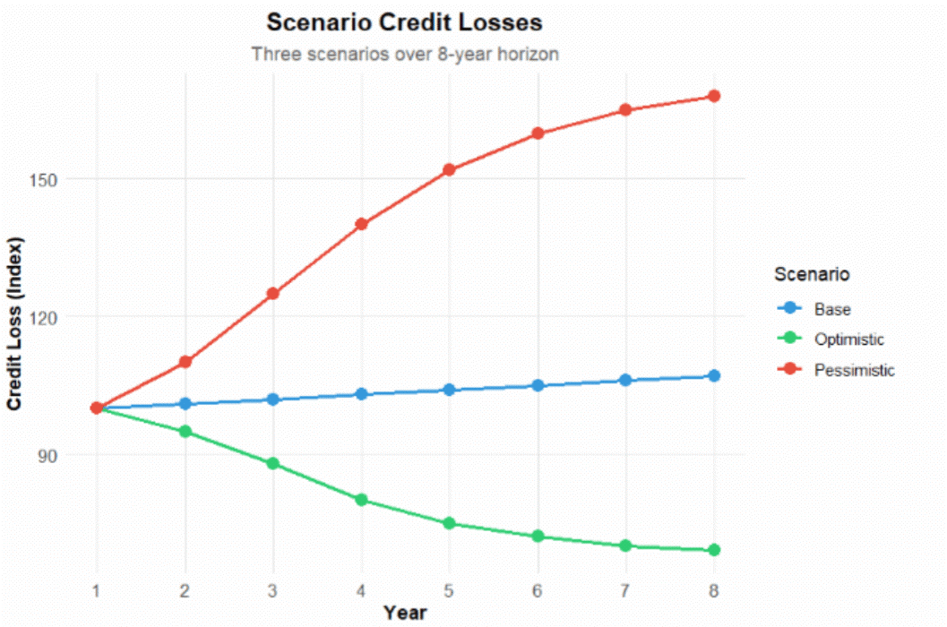
Since we’re modeling losses, the pessimistic (red) curve is above the other two curves, with the baseline scenario in the middle. This is logical. Or is it? Before we answer this question, let’s first have a look at the governance around the macro scenarios.
Macro Scenarios’ Governance
Each macroeconomic driver is expressed in terms of three time series, for the pessimistic, base and optimistic scenarios. For each scenario, it has a forward looking horizon that is sufficiently long for capturing the direction of the losses for the remaining maturities in the portfolio.
Common macro drivers that banks consider are GDP, unemployment, inflation, house price index, and selected raw material and food indices. In principle, any indicator could work for which it is has been established that historically, the point-in-time PD and LGD depend upon it. The macro indicators are sourced from reputable internal or external sources, e.g. central banks.
Once the macro drivers have been selected (suppose GDP, unemployment and food price index), the forecast series are sourced and inspected. It is important that the bank has a coherent overall narrative about the future macro state-of-the world. Such a narrative explains how, e.g., in the pessimistic scenario, one sees decreasing GDP, rising unemployment and progressing scarcity of food due to environmental and supply-chain disruptions which lead to increasing food prices.
This overall narrative is applied to the portfolios through the collected forecasts of the macro drivers. We will then see that, given the pessimistic scenario, the PDs and LGDs will increase, leading to high projected losses. The optimistic scenario will lead to lower losses, and the base scenario will have a position in between.
It is important that the bank has only one overall narrative. It has to be able to explain to internal and external supervisors how it views the future macro directions and how it applies these to its portfolios in order to derive the future scenario losses.
Conversely, if the bank would use a different scenario set, say, for the retail portfolio than for the business portfolio, that would be impossible to substantiate. The provisioning could then not be tied back to one overall macro narrative. The economic actors of the retail and business portfolios do not live in separate worlds, they interact in the same macroeconomic environment; hence, for provisioning, the pessimistic, base and optimistic scenarios have to be deployed coherently across all portfolios.
Generating Counterintuitive Results
We are now positioned to go back to where we left off. The bank has established a set of relevant macro drivers, in our example: GDP, unemployment and food prices. For the optimistic scenario, GDP increases, unemployment decreases, and food prices decrease. For the pessimistic scenario, the directions are reversed, and for the base scenario the variables roughly stay the same.
Let’s assume that for this bank, for the retail portfolio, this works out fine. The pessimistic scenario increases PDs since consumers earn less, they have less affordability for servicing their loans, they may even become unemployed, and they pay more for their food. The same is true for almost all business portfolios: For the pessimistic scenario, losses drift upwards, while for the optimistic scenario they drift downwards, exactly as they should, as illustrated in Figure 1.
However, our example bank has one business portfolio that behaves differently. It benefits from increasing food prices. And it benefits to such an extent that the other macro indicators (GDP, unemployment) cannot compensate for this. The reason is that this business portfolio lends to food producers. If we suppose that these producers are not affected by macro disruptions of the supply chain (e.g. they produce for local and nearby markets), then these firms will structurally and significantly reap the benefits of increasing food prices.
Of course, the impact in this example could be weakened. The increase in food prices could be mitigated by the lower incomes (lower GDP) that is also part of the macro scenario. But it is probable that in such scenarios, the increase in food price is the dominant and most immediate factor for the food producers, so that, at the end of the day, they benefit from the situation as expressed in the pessimistic scenario.
If we then hold on to the principle that there is only one future state of the world (expressed in the pessimistic, base and optimistic scenarios), in our example, the bank ends up with all-but-one portfolios behaving as illustrated in Figure 1; and one portfolio, the business portfolio lending to food producers, having an exceptional IFRS 9 profile with lower losses for the pessimistic scenario than for the optimistic scenario – the inverse picture of Figure 1.
Zooming Out
Although in cases like this, the inverse IFRS 9 profile is the result of logical premises and reasoning, the bank may have a hard time explaining this outcome to the supervisor. But the anomaly is justified once the bank starts with the overall macro narrative and then substantiates step-by-step how it derives the portfolio losses according to the IFRS 9 standard.
Another way of understanding the situation is by zooming out and realizing that, within the broader FRM discipline, this is not that exceptional at all. The business portfolio for food producers functions as a real hedge, and hedges are very common in other FRM areas, for example market risk.
Notwithstanding this broader picture, I do expect banks worldwide to encounter the described phenomenon in exceptional cases, and explaining why the pessimistic scenario leads to lower losses will not always be easy.
Dr. Marco Folpmers (FRM) is a partner for Financial Risk Management at Deloitte the Netherlands.
Topics: Counterparty, Modeling, Model Risk