Considering one of the most difficult items to grasp within credit risk modeling, I am reminded of what St. Augustine said about the question, “What then is time? If no one asks me, I know; if I wish to explain it to one that asks, I know not.” (Confessions, Book XI)
For financial risk professionals, this applies to the asset correlation.
It is easy enough to give a high-level description of this asset correlation as it functions within IFRS 9. All exposures belong to a specific PD (probability of default) rating grade. Each grade has fitted PD values that change, conditional on the expected future macroeconomic environment.
When better economic times are foreseen, the PDs decrease, and when the conditions turn more unfavorable, the PDs increase.
This means that future PD trajectories, or PD curves per rating grade, will depend upon macro developments, often measured by GDP growth, asset prices and unemployment.
Marco Folpmers
Usually banks model these PD curves per rating grade. The projected point-in-time PDs depend then on the starting PD (the through-the-cycle PD) and the expected macroeconomic developments. The level of dependence is often measured with the help of the so-called “asset correlation.” High asset correlation introduces large swings in the PD curves as they respond to the macroeconomic conditions, and, vice versa, a low asset correlation will lead to a more stable and less fluctuating PD curve.
The mechanism through which macro developments and through-the-cycle PDs are translated to point-in-time PDs is often the Vasicek formula. This formula is also used in the Basel rule set to compute the risk-weighted assets according to the IRB (internal rating based) approach for credit risk.
This, then, is the high-level description of the asset correlation. However, once introducing further refinements, the concept becomes a lot harder to grasp with the risk of ending up with a rating system that violates fundamental design properties. Let’s unpack this carefully in the remainder of this article.
Increasing Asset Correlations Across PD Grades
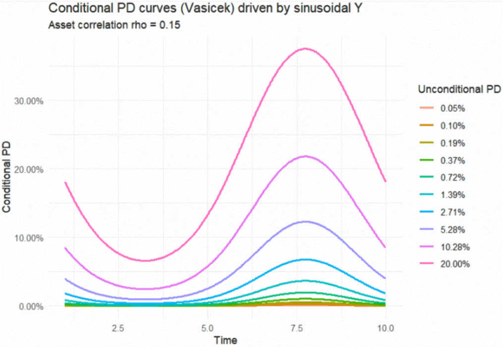
For a moderate asset correlation of 15%, the PD curves per grade can be depicted as in Figure 1. A rating system has been used with 10 grades, running from a minimum PD value of 5 basis points to the maximum of a 20% PD. The calibrated, through-the-cycle PDs per rating grade are initialized as an exponential curve.
Figure 1: A System of Conditional PD Curves

Progressing in time from left to right, we see that the projected PDs per grade show the influence of the macro economy (modeled as a sinusoidal driver). The graph first shows a favorable economic environment, with decreasing PDs, and then an unfavorable environment with increasing PDs. We also see how the asset correlation affects the curves proportionally while using one fixed asset correlation (rho = 15%). The swings in the larger PD grades are higher than those at the bottom part of the graph for lower PD grades.
While using one fixed asset correlation is difficult enough, the Basel RWA formulas introduce a further complexity, and that is an asset correlation that varies across PD grades.
In the Basel RWA formula, the asset correlation for corporate exposures decreases across grades, from 24% to 12%. Apparently the Basel Committee professionals who engineered the capital and asset correlation formulas had reason to believe that the dependence on the macro environment decreases for higher PDs. The overall reasoning is that, for high-quality borrowers (low PD), the default risk is systematic rather than idiosyncratic, so that they default because of a systematic crisis rather than through specific factors (such as quality of management). This would explain a higher rho for lower PDs.
There are different views. A 2025 Global Credit Data report (building on an earlier one by the European Banking Authority) found that asset correlations do indeed change across rating grades, but they generally show an upward trend instead of a downward movement. This means that he higher PD grades are actually more sensitive to macroeconomic swings than lower PD grades.
This has great implications for IFRS 9 modeling. If indeed PD curves are established that have these kind of swings, it may even invalidate the whole IFRS 9 modeling system if one isn’t aware of the consequences, as we will demonstrate.
“Dripping Phenomenon”
Take a new look at Figure 1; approximately at Time t = 3, all PD curves reach their minimum (and the economic environment is the most favorable). If the upper curves then suffer more of a downswing than the curves immediate below, technically they may cross. This means that the upper curve “drips into” its lower neighbor. Could this happen in our system with the 10 rating grades?
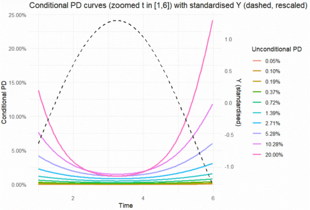
In our system of 10 rating grades, we need to stretch the asset correlations considerably for this to happen, using asset correlations ranging from 2% for the lowest PD grade (unconditional PD = 5 bp) to 40% for the highest PD bucket (unconditional PD = 20%).
In Figure 2 we show the standardized macro driver (the dotted line) and the 10 PD curves using these asset correlations. When we zoom in on the start of the figure (the economically favorable regime), we see that indeed the curve of the highest PD grade (20%) swings lower than the PD curve of its neighbor below (PD = 10.28%) and actually crosses it.
Figure 2: The Dripping Phenomenon

From a credit risk point of view, this phenomenon is impossible to explain. It is a clear violation of so-called monotonicity. The PD values of each rating bucket have to increase monotonically as risk increases across these buckets for a proper risk measurement set-up. Any design that leads to a violation of monotonicity is wrong on principle.
Parting Thoughts
From a practical perspective, our recommendation is that banks that use advanced IFRS 9 modeling techniques and apply increasing asset correlations across grades, should test extensively whether the resulting PD curves make sense and comply with important design principles such as non-violation of monotonicity in the PD system.
The difficulty is that IFRS 9 formulas are often applied mechanically, while updates of fitted asset correlations can have unforeseen consequences, of which the violation of monotonicity is only one example.
As in the Augustinian saying, professionals may have a general understanding of asset correlation within credit risk, but to produce a fully developed view on how asset correlations impact IFRS 9 models and their intermediate and end results is very hard.
In this article we only scratched the surface, ignoring many other complexities surrounding the asset correlations, such as how to measure them (using market data or default data?), their instability in time and their interaction with other modeling components (especially the migration matrix).
FRM professionals and especially validators are advised to closely inspect not only the IFRS 9 end results (the ECLs – expected credit loss) but also all the intermediate steps, such as the derived PD curves.
Marco Folpmers (FRM) is a partner for Financial Risk Management at Deloitte the Netherlands. Dr. Folpmers wishes to thank Ioannis Banatas (Deloitte Alexander Competence Center, Thessaloniki, Greece) for his insights on asset correlations within IFRS 9.