
Proper back-testing is crucial for any bank that submits its PD and LGD models to its supervisor for approval. To meet the requirements of regulators like the European Central Bank (ECB), banks must assess the predictive ability of their PD estimates to determine whether they constitute reliable forecasts of default rates.
Today, many European banks back-test PD through the so-called Jeffreys test - a predictive ability test developed by Harold Jeffreys, a renowned British mathematician, geophysicist and astronomer. This back-test, however, is not without its issues, and banks must plan carefully to overcome its beta distribution and PD estimation challenges.
Let's now walk through the fundamentals of the test and weigh its pros and cons.
The Jeffreys Test for Predictive Ability
The Jeffreys test can be applied both at the single rating-grade level and at the portfolio level. While we will focus on the single rating-grade level, our analysis is generalizable to the application of the Jeffreys test at the portfolio level.

Essentially, the test checks whether the observed default rate is in line with the default rate assigned to a specific PD rating grade - e.g., PD = 2%. It relies on evidence of collected defaults and non-defaults gathered from a historical database.
Under the Jeffreys test, true PD is seen as an unknown population parameter: say,  . With the help of the sample evidence, a confidence interval is established for this unknown parameter. This confidence interval is interpreted as a probable interval in which the true (but unknown) population default rate resides. The probability that the unknown parameter is within the interval is 1 minus the confidence level - i.e.,
  .
.
While the population parameter will continue to be unknown, with the help of sample information, we can at least establish a confidence interval for the parameter. For increasing sample sizes, the confidence interval will be increasingly smaller, indicating more and more precise knowledge about the value of the unknown population parameter.
Since the Jeffreys test is a one-sided test, it has a one-sided confidence interval, and there's only one rejection area. The only concern with this test is that the bucket PD may be too low.
A Simple Example
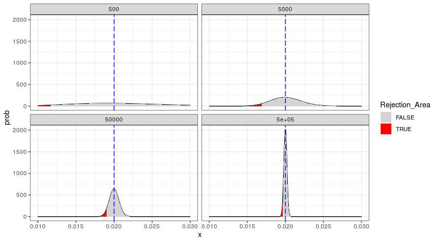
In the graph (Figure 1) below, we have illustrated the one-sided confidence interval ( ) for the Jeffreys test. The dashed blue vertical line indicates the bucket PD (2%). The intervals have been construed by using sample outcomes (that also have a default rate of 2%) for several (increasingly larger) sample sizes, which are depicted in four panels.
The figure on the top-right illustrates the situation for a sample size of 5,000 loans, in which (by construction) 2% (i.e., 100) were actual defaults and 98% (4,900) were non-defaults. In the figure, we see a confidence interval for the true (but unknown) population parameter - including a rejection area in red.
In practice, this means that, with the help of the evidence from the test, a bank can accommodate values for the bucket PD as low as the minimum value in the grey shaded area - given that the sample outcome contains 2% defaults. Below that value, the red area (i.e., the rejection area) starts; this is where the test fails, and one must conclude (based on evidence from the sample) that the bucket PD is too low.
Figure 1: Confidence Intervals for the Jeffreys Test
(4 Samples of Increasing Size)
The bottom line is that it is acceptable to use a bucket PD that is lower than the default rate in the sample (so, in our case, a bucket PD that is lower than 2%) - but only up to a certain extent.
In our example, we see that the bucket PD of 2% (the dashed blue line) fits nicely in the acceptance (grey) area of the distribution. This should be the case since, in this example, the sample default rate is exactly equal to the bucket PD (both are 2%) by construction.
When looking at all four charts in Figure 1, we see that the probability density function becomes more and more narrow as we increase the sample size, and the evidence consistently shows a 2% default rate. The larger the sample size, the more certain we are about the unknown value of the population parameter . The population parameter, although “unknown,” can be assessed with an increasing level of precision, since we gather more and more evidence for increasing sample sizes.
If we were to grow the sample size beyond the examples in Figure 1, the density function would further “collapse,” ultimately leading to a “degenerate” distribution that shows only a spike at 2% (with infinite probability). In that case, the population parameter would no longer be unknown.
Background: Bayes and Beta
The technique with which the Jeffreys confidence interval is built is a beta distribution that uses two parameters,  and
and  . Parameter can be interpreted as the sample evidence for defaults, while parameter covers non-defaults. So, in principle, the top-right chart in Figure 1 depicts a case in which the sample of 5,000 loans contained 100 defaults and 4,900 non-defaults.
However, there is a small nuance. When applying the beta distribution, it is possible to adjust the parameters and with so-called prior information.
There's much discussion among statisticians about the proper prior information to use when applying the beta distribution, where  (the “zero prior”);
  ; and
; and  have been proposed. It's safe to say that, as it relates to meeting ECB guidelines, the Jeffreys prior () applies.
Closeness: Boundaries Between Defaults and Non-defaults
When increasing the sample size, the density function starts to collapse, and therefore the defaults boundary between the red rejection area and the grey area shifts to the right. This is visible on the bottom-right panel of Figure 1, which is magnified in the figure below.
Figure 2: Confidence Interval for the Jeffreys Test
(Sample Size = 500,000)
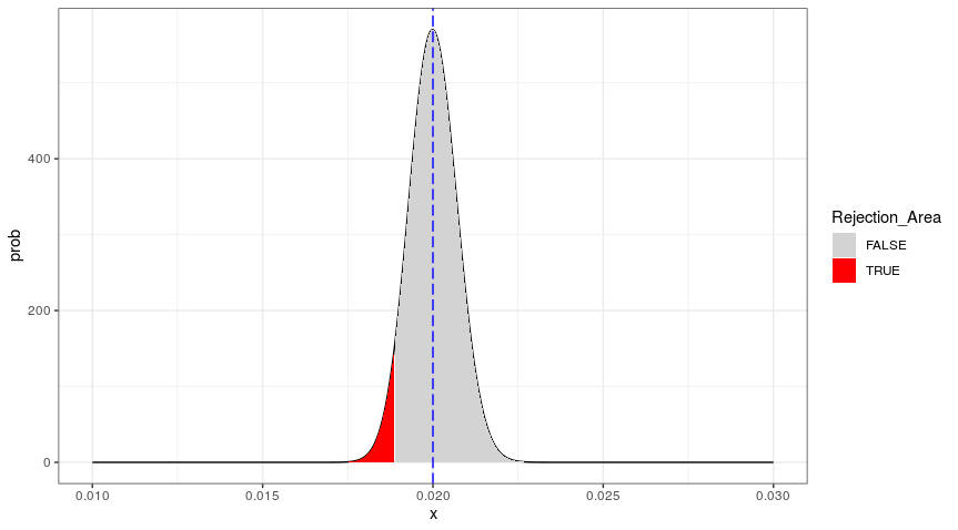
The boundary in this graph, between the red area and the grey area, is 1.8874%. (The exact boundary is part of the grey area, since, for inequality tests, the equality is always included in the null hypothesis.) In this case, the boundary is already very close to the bucket PD of 2%, and we can express the closeness as the boundary value (for  ) divided by bucket PD - i.e., 1.8874% /2% = 94%.
The higher this “closeness,” the harder it is to accommodate a bucket PD that is smaller than 2%. In the case depicted in Figure 2, the evidence of this sample of 500,000 observations would not allow a bucket PD equal to 1.88%. However, a smaller sample from the same population (population default rate is 2%, by construction) would allow a bucket PD equal to 1.88%, given a smaller red rejection area.
For larger sample sizes, the minimum acceptable bucket PD comes closer to the population default rate. For an infinite sample size, the minimum acceptable bucket PD would be 100% of the population default rate. Under that scenario, the minimum acceptable bucket PD would be close to 100% of the population default rate.
For smaller sample sizes, there is more “leeway.” Since the rejection area is smaller, the closeness of the minimum acceptable PD to the population parameter is amply below 100%, and some bucket PD values below the population parameter can be accommodated.
In the figure below, we demonstrate that the closeness of the boundary increases toward 100% for increasing sample sizes.
Figure 3: Closeness for Increasing Sample Sizes for Bucket PD
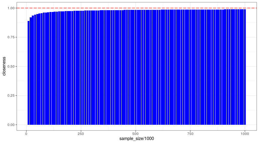
To ensure that the bucket PD of 2% does not end up in the rejection area, it is important that the closeness of the boundary remains below 1. However, for the sample loan sizes (which are not unrealistic for retail portfolios), the red area (see above) comes very close to the bucket PD value. When this occurs, bucket PD values below the population parameter can hardly be accommodated.
Perverse Incentives
In practice, the increasing closeness of the rejection area to the PD bucket value might lead to a situation in which a bank has a rating grade that has an (unknown, but expected) population default rate of = 2%. Under this scenario, to prevent failing the Jeffreys test, banks “play it safe' and use a bucket PD that is overestimated. In this situation, it is preferable for the rating grade to be assigned to a bucket PD that is slightly larger, given the closeness of the rejection area for large sample sizes.
The assignment of a higher bucket PD is prudent, because it helps to prevent the failure of the Jeffreys test - especially given the possibility of some short-term volatility in the default rate.
As we have demonstrated, under the Jeffreys test, the beta distribution of defaults can collapse for large sample sizes. Banks will need to take this into account by establishing a “safe” bucket PD, which should aim to be slightly above the suspected population mean.
The Jeffreys test, in short, introduces in practice an upward bias to the bucket PD. This is a remarkable result for a test that is the most important tool for establishing the predictive ability of the PD rating system.
Dr. Marco Folpmers (FRM) is a partner for Financial Risk Management at Deloitte Netherlands. He is also a professor of financial risk management at Tilburg University/TIAS. He wishes to thank Sanne van den Brink (M.Sc.) for kindly providing feedback on an earlier draft of this article.