
The Jeffreys test is the most important diagnostic tool for assessing the calibration of the bucket probability of default (PD). However, it actually has a wider range of applications.
Potentially, this test can also be applied to validate, e.g., loss given default (LGD) and the cure rate - the fraction of loans that recover from default status to non-default. Prior to examining how this test can be applied elsewhere, we need to discuss the challenges it presents and understand its mechanics, particularly: (1) its statistical definition, as a one-sided hypothesis test; and (2) the dynamics of the assumed beta distribution of the observed default rate.
We'll now examine these mechanics, and then discuss the adjustments that must be made when a risk manager expands the test to other credit-risk use cases.
Breaking Down the Mechanics
The Jeffreys test assesses whether the bucket PD (i.e., the PD of the bucket to which a given exposure is assigned) is in line with the empirically observed number of defaults in this bucket.

Under a typical Jeffreys test, loans are allocated to a certain PD bucket, establishing the number of defaults D within a total number of N loans within this bucket. For a given backtesting timeframe, and, based on this evidence, a confidence interval is established for acceptable values of the bucket PD. The acceptable values are either probable values (given the evidence) or conservative values.
Statistically speaking, for a given PD bucket, there's an unknown population probability of default π. For this unknown PD, under the Jeffreys test, a one-sided confidence interval is established with the help of the evidence - i.e., the number of defaults D found in the N loans that have been allocated to this bucket within the scope of the backtest.
The rejection area is on the left-hand side of the confidence interval. This means that only levels of π below a certain threshold are rejected; high values of π are not rejected.
Regulatory requirements present another challenge for users of the Jeffreys test. For example, in its instructions for reporting the PD validation results of internal models, the ECB describes the null hypothesis as follows: “The null hypothesis that the PD applied in the portfolio/rating grade at the beginning of the relevant observation period [should be] greater than the true [one-sided hypothesis test].”
However, when testing one-sided hypotheses, the equality sign is always part of the null hypothesis. So, at the risk of sounding pedantic, the ECB should have included the “equal to” in its null hypothesis for PD validation.
Jeffreys' Bucket PD Assumptions
One final point to consider with respect to the mechanics of the Jeffreys test is the assumption it makes for bucket PD. Under the test, when we allocate loans to a PD bucket with which a certain PD is attached, we are implicitly making the assumption that the bucket PD (for a specific bucket) is a reasonable value for the unknown population parameter π.
So, how does this work in practice? Let's assume that we're working with loans that have been allocated to a PD bucket, with PD equal to 1%. Under this scenario, the null hypothesis is H0: 1% ≥ π. Suppose also that, while performing the backtest, we have come across one default out of 250 loans (so, D = 1 and N = 250).
This evidence leads to the specification of a beta distribution in which α = D + 0.5 = 1.5, and
b = N – D + 0.5 = 249.5. (In these equations, the “0.5” parts are the so-called “Jeffreys priors” that we've discussed on a previous occasion).
Let's denote the beta probability density function by f(p;a,b) and the corresponding beta cumulative distribution function by F(p;a,b). This beta density (with α = 1.5 and b = 249.5) is depicted below, where the vertical dashed line indicates the value of the bucket PD (1%).
Figure 1: Beta Density for the Jeffreys PD Test
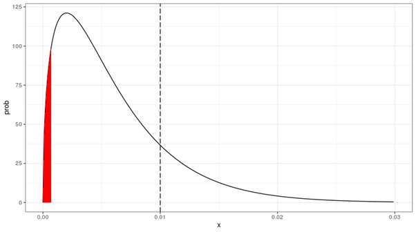
The red area in Figure 1 shows the rejection area for a one-sided confidence level of 5%. In this example, the limit of the red area is equal to 0.0007 (since F(0.0007;a,b) = 5%).
The bucket PD is not in the red area, so we can assume that a bucket PD of 1% would either be probable or conservative. Equivalently, one can calculate the probability mass at the left side of the indicated value of 1%; this probability mass turns out to be 83.0% (= F(0.01;a,b)), which is amply above the confidence level of 5%.
Since this is a one-sided test, there is no problem with bucket PD values, which are very much in the right-hand tail. In the above example, a PD bucket value of 20% will not be rejected - although, given the empirical evidence, it is highly unlikely to be close to the true (but unknown) population parameter π. It is therefore important to realize that while the Jeffreys test is a valuable tool for PD calibration, it should not be used to assess accuracy, since values that are way off (e.g., 20%) can still pass the test.
Expanding to Other Use Cases
In practice, it is attractive to apply the Jeffreys test to other use cases within credit risk - e.g., a credit conversion factor (often part of an EAD model), or the LGD or the cure rate (a sub-model for the LGD). However, when doing so, it is important to carefully adjust the formulas.
Since this is a one-sided test, it makes a difference whether one assesses a parameter for which it is true that “the lower the better” (as with the default rate) or “the higher the better” (as with the cure rate).
Let's now consider an example related to the cure rate. Suppose that, within 200 defaults, we've found 180 cures (so, so, C = 180 and N = 200). Suppose also that the cure rate in use is equal to 92%.
In this case, it is immediately clear that the established cure rate is a bit on the high-side (i.e., optimistic), since the empirical evidence points to a cure rate of only 90% (or 89.8%, when taking into account the Jeffreys priors and calculating the mean as α / α + b). So, the question is: will the cure rate in the Jeffreys test be too high?
Figure 2: Beta Density for the Jeffreys Cure Rate Test
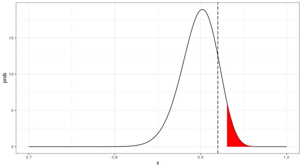
In Figure 2, the rejection area is now on the right-hand side of the density. The formulas that were applied above therefore need to be slightly adjusted. The limit of the rejection area is equal to 0.9307 (since 1 - F(0.9307;a,b) = 5%). Since 92% < 93.07%, there's no need to reject the null hypothesis.
Equivalently, one can calculate the probability of having a cure rate equal to 92% or higher as 14.88% (1 - F(0.92;a,b)), which is above the 5% confidence level.
As a shortcut, there is an alternative approach possible, where formulas for PD need not be adapted. For example, we can reformulate the Jeffreys test from the beginning, with respect to “the lower the better.” In this example, we can convert the cure rate to a no-cure rate. Consequently, within 200 defaults, we find 20 no-cures (so NC = 20 and N = 200, and α = 20.5 and b = 180.5).
Since the assumed cure rate = 92%, the null hypothesis is that the no-cure rate of 8% is acceptable. We can use the unadjusted formulas and conclude that, as 14.88% (= F(0.08;a,b)) is above the 5% confidence level, the null hypothesis need not be rejected. Therefore, the no-cure rate of 8% is acceptable, as is the cure rate of 92% in the original hypothesis.
Parting Thoughts
Applying the Jeffreys test to use cases outside of PD (including the cure rate) is potentially beneficial, but also tricky. The table below summarizes the factors that must be considered, taking into account the conservative assumption underlying the null hypothesis, the location of the rejection area, and the direction of the null hypothesis.
Table 1: Summary of the Jeffreys Test for Alternative Use-Cases
|
Case: |
Default rate |
Cure Rate |
No-Cure Rate |
|
Conservative: |
The lower the better |
The higher the better |
The lower the better |
|
Rejection area, on which side of the distribution? |
On the left-hand side |
On the right-hand side |
On the left-hand side |
|
Direction of H0: |
Bucket PD ≥ True PD |
Cure Rate in use ≤ True Cure Rate |
No-Cure Rate in use ≥ True No-Cure Rate |
The Jeffreys test is a powerful tool. However, it can only be applied effectively to, say, LGD and the cure rate after the implications of the one-sided test are considered.
Dr. Marco Folpmers (FRM) is a partner for Financial Risk Management at Deloitte Netherlands