Probability of Default: The Pluses and Minuses of Transition Matrices

Transition matrices measure the transition probabilities for credit-risk ratings over specific time intervals, and are among the most vital tools at the disposal of a credit risk manager for projecting probability of default (PD) evolution. But these matrices are more complex than they seem to be on the surface, thanks in part to obscure momentum and reversal phenomena.

A transition matrix tells us what the PD transition probabilities are for each PD rating within a given portfolio (e.g., SMEs). It provides the probabilities for whether the rating will remain the same, shift to a better (upgrade) or worse (downgrade) rating, or even jump immediately to default status. (After a loan has been repaid or written off, it's also possible, of course, that its exposures under a transition matrix will be moved to a 'closed' status.) While the time interval for each transition matrix varies, transitions after a quarter of a year or a full year are projected most often.

Regulators typically mandate the use of transition matrices. The ECB, for example, asks banks to provide transition matrices for each of their portfolios, while also requiring the application of a number of tests. Usually, these are stability tests that require a bank to demonstrate that the majority of its PD rating migrations are limited to small steps. Each bank, moreover, also needs to show a reasonable number of negative shifts (rating downgrades), as compared to positive shifts (rating upgrades).

In technical terms, each (single) transition matrix for credit-risk ratings is supposed to be a first-order Markov chain that can predict the future. In this first-order Markov world, history is not relevant. This means that all exposures in, say, current grade (2) are projected to future credit grades, regardless of how they ended up in current grade (2).

However, for credit risk, this is quite a strong assumption, partly because history is demonstrably important. For example, M. Malik and L.C. Thomas found in their 2012 paper that for a consumer portfolio, a second-order Markov chain is needed. More recently, G. dos Reis, M. Pfeuffer and G. Smith (2020) found “non-Markovian” rating movements for corporate portfolios.

Opening Up the Transition Matrix

Let's now have a look at a (very) simple credit-risk ratings transition matrix in which there are four non-default states and one default state. State (1) is the best state (associated with the lowest PD), whereas state (4) is the worst state (associated with the highest PD).

Suppose that the first-order yearly rating transitions are as follows, for exposures currently in state (2):

Table 1: Transition Probabilities for Current State (2)

The probability that the exposures in current state (2) remain in state (2), across the one-year time interval, is high (89.5%). This probability, which is typically on the main diagonal of the migration matrix, is shown in grey. We also see that the default probability that is associated with this state is 1%, and that, after a year, 4% of the loans are closed.

The remainder of the data in the table provides us with the transition probabilities to the other (non-default) states. As a simple stability test, based on this information, we can calculate that the probability that the rating migration stays within a [-1, 1] range is 93.8%.

The table does not explain how the exposures in state (2) are built up. As we explore their migration path over the past 12 months, it's very hard to say whether the exposures in state (2) have predominantly been upgraded from states (3) and (4) or downgraded from state (1). Indeed, this important information is lacking, which means that any patterns (i.e., previous downgrades or upgrades) are completely hidden from us in a typical transition matrix.

In the table below, a breakdown is provided of the stage 2 transition probabilities for the portfolio of loans in our example (one-year time interval) transition matrix.

Table 2: A Breakdown of Transition Probabilities for Current State (2)

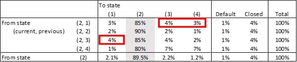
It is clear from the above data that the first table only provides an aggregation of the information. Upon closer inspection, we can conclude that Table 2 does not differentiate with regards to the default and closed probabilities (1% and 4%, respectively). However, it does differentiate for the gray scenarios (the probability that the credit-risk rating remains in state (2)), since the probability to remain in state (2) is significantly higher for previous state (2) exposures. “Persistence” is a good descriptor for this trend.

More interestingly, downgrades in Table 2 are not mirrored by offsetting upgrades. An exposure that was downgraded previously from state (1) to state (2) has a 7% probability of a further downgrade toward states (3) and (4) (see upper-red rectangle). However, an exposure that was upgraded from state (3) has only a 4% probability of a further upgrade to state (1).

This is an important phenomenon. For downgrades, we see “momentum” - i.e., previous downgrades can lead up to further downgrades. This is important information, especially if this momentum is not mirrored by a (compensating) momentum in the upgrades. Consequently, in this example, we witness asymmetric momentum.

The opposite of momentum is reversal. In the context of transition matrices, a reversal happens when transitions from current states to previous states are probable. Typically, a reversal occurs when rating systems are technically unstable - i.e., (1) if the creditworthiness is expressed in a score that is then converted to a grade with the help of bandwidths per grade; and (2) if an exposure is persistently scored at the boundary between two bandwidths. This combination of circumstances may lead to a “switching back-and-forth” type of behavior between the two rating grades.

It is important to identify symmetric and asymmetric momentum empirically in the transition information. Asymmetric momentum for downgrades is a dangerous phenomenon, and it is interesting to try to link this phenomenon to systematic drivers - e.g., the state of the economy.

During recessions, it is possible that there's more downward momentum than during benign economic times. This may also apply to the current COVID-19 era.

Parting Thoughts

There's more behind a simple transition matrix for credit-risk ratings than meets the eye. In this article, we have explained the impact of phenomena (like asymmetric momentum, reversal and persistence) on PD rating transitions.

Momentum is an especially important factor to identify, as it can reinforce downgrades from the past. Even more can be gained by acknowledging that momentum is probably not stable across time and may be related to recessionary macro circumstances.

Dr. Marco Folpmers (FRM) is a partner for Financial Risk Management at Deloitte Netherlands. Thanks are due to Hao Zhou, who kindly reviewed an earlier draft of this article.