The Skewed Generalized T Distribution: A Swiss Army Knife for Tail Risk

Every risk professional knows that price shifts can widely diverge. Daily or weekly returns can go up or down in a more significant way than predicted by a normal distribution. When assessing and analyzing asset price return data, this phenomenon - known as fat tails or leptokurtosis - is easily identified.

However, there is no standard for modeling these tail-risk events, and financial institutions still have work to do to determine which methodology may work best - particularly during highly stressful periods (like the COVID-19 pandemic or the Global Financial Crisis) where we have seen some extreme movements.

A t distribution - regarded as a more generalized distribution than a normal distribution - is sometimes used with low degrees of freedom (DF) for the modeling of fat tails for financial return data. One can arrive at a higher leptokurtosis by lowering the DF of the t distribution.

Consequently, the more generalized t distribution is a better candidate for capturing the properties of financial return data than the normal distribution, which has infinite DF. However, neither the generalized t distribution nor the normal distribution considers the fact that the empirical financial return distributions are often not only leptokurtic but also asymmetric - i.e., they display heteroskedasticity.

Therefore, an even more general distribution for modeling financial return data is needed. Though it is not often applied in practice, the Skewed Generalized T Distribution (SGT) is a good solution. The SGT has five parameters: mu (for location), sigma (for dispersion), lambda (for heteroskedasticity), and p and q (for determining the leptokurtosis).

With the help of SGT and proper specification of these five parameters, one can generate many known distributions - not only the normal and t distributions but also the Laplace, Cauchy and uniform distributions, to name a few.

For these reasons, the SGT is regarded as the “Swiss Army Knife” for the modeling of financial return distributions. It is a flexible distribution model that has enriched the financial risk manager's toolkit significantly since its creation by Panayiotis Theodossiou in 1998.

S&P 500 Index Returns

For a practical application of fat-tail modeling, we can use the daily log returns on the S&P 500 index, via downloading data from January 2017 to February 2021 (1,045 business days).

The daily log returns are depicted below (see Figure 1). They show the usual trends in financial return data, such as volatility clusters. As readers can see, volatility is higher than usual during certain timeframes - particularly amid the start of the COVID-19 crisis in the first quarter of 2020.

Figure 1: S&P Log Returns

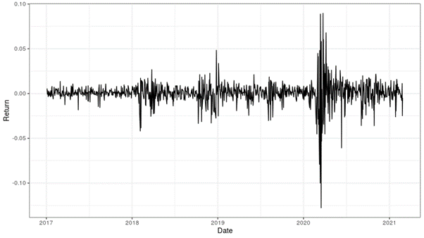
This leptokurtic example (excess kurtosis = 21 bp) also demonstrates the general asymmetry of financial return data. The negative returns (which exceed -10%) in Figure 1 are more acute than the upward returns. Indeed, on average, the downward returns (with a mean of -80 bp) are more pronounced than the upward ones (mean = + 70 bp). However, the fact that upward returns occur more often (590 days) than negative returns (454 days) somewhat counters the downward trends - at least from investors' point of view.

It's also interesting to note that, in Figure 1, there are six returns smaller than -0.05 and five returns larger than +0.05. Given that the standard deviation is 129 bp, these 11 extremes represent at least 3.8 sigma events in only 1,045 business days.

These results demonstrate that a normal distribution fit for modeling fat tails is not a good idea. The graph below (which depicts cumulative distribution functions) also drives this point home.

Figure 2: Empirical and Fitted Normal Distributions

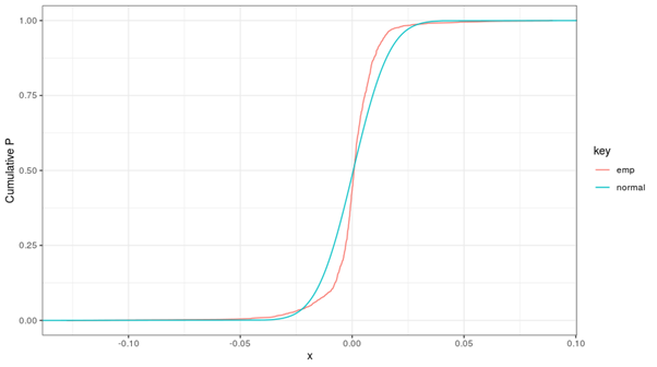
In Figure 2, we see that the fitted cumulative normal distribution does not properly align with the empirical distribution of the daily log returns. The symmetrical normal distribution is not able to capture the asymmetry of the empirical distribution: e.g., the area between the two curves is different between the left- and right-hand sides of the cross-over point (close to 𝓍 = 0). Furthermore, the normal distribution is clearly insufficiently fat-tailed.

The requirements for a modeled distribution for the empirical log returns include not only fat tails but also asymmetry. Therefore, it makes sense to look for a more generalized t distribution that can not only accommodate leptokurtosis but also account for some asymmetry - or at least the heteroskedasticity. It is then a logical step to turn to the SGT.

As previously mentioned, this distribution contains five parameters. These five parameters can be fitted to the time series at hand with the help of a maximum likelihood procedure (e.g., sgt.mle in R). The result is depicted below.

Figure 3: Empirical and Fitted SGT Distributions

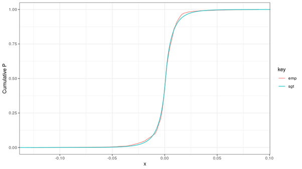
The fit depicted above is good - not only in the “body” of the distribution but also for the tails, the part of the distribution in which most risk managers are particularly interested.

Parting Thoughts

Proper modeling of returns of financial asset prices is crucial in many domains of financial risk management. For an investment portfolio, one needs to have a good view of the value changes that can be expected within a specific timeframe. Since tail risk plays an instrumental role in risk management (via, e.g., helping a bank determine its capital requirement), models need to be able to capture tail events properly.

There is also a direct link between fat-tail modeling and credit risk. Exposures to funds (like mutual funds and hedge funds) have a probability of default (PD) that is determined by the net asset value of that fund. Fat-tail modeling can help a bank figure out the PD of a fund, which is the chance that returns will be so unfavorable that the fund's net asset values drop below zero.

For different types of assets on the balance sheet, the preferred modeling approach is to fit univariate SGT distributions for the asset price log returns, and to then link these through a copula function.

Dr. Marco Folpmers (FRM) is a partner for Financial Risk Management at Deloitte Netherlands and a professor of financial risk management at Tilburg University/TIAS. He wishes to thank Roland Walles (M.Sc.), who kindly reviewed an earlier version of this article.