How to Improve LGD: Unlocking the Generalized Area Under the Curve

It is difficult to gauge the performance of loss-given default (LGD) models, partly because it’s hard to discern the difference between estimated and realized LGD. But the generalized area under the curve (gAUC) can help close that gap. In fact, gAUC is the most important metric for assessing the performance of an LGD model.

The assessment of estimated vs. realized LGD is more complex than it is for probability of default (PD). For PD, a model outcome (creditworthiness score) needs to be set off against a binary dependent variable: i.e., a “Yes/No” for default. For LGD, this comparison between estimated and observed values is more complex, and therefore requires gAUC – an extended version of the area under the curve (AUC) metric.

Marco Folpmers

Before we discuss the calculation of gAUC, it’s important for us to understand the differences between the calculations for realized (or observed) and estimated LGD.

The estimated LGD is either a score between 0% and 100% or a specific parameter (e.g., “between 10% and 20%”) on this scale. The observed LGD is a loss realization that is typically a score between 0% and 100%; for atypical cases, some procrastination is needed, since loss rates can be negative or exceed 100% of the exposure.

The usual way to compare estimated LGDs () and realized LGDs () is to impose an ordinal scale of LGD buckets. Under this approach, both estimated and observed LGDs must be converted to these buckets, according to the following (ECB-driven) bucketing system:

• LGD Segment 1: loans with ;
• LGD Segment 2: loans with ;
• LGD Segment 3: loans with ;
• …
• (10% LGD steps from Segments 4 to 11);
• …
• LGD Segment 12: loans with .

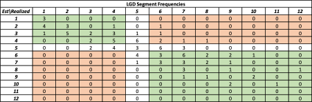
After the application of this bucketing, we end up with an LGD dataset for testing purposes, consisting of loans with an estimated LGD bucket and a realized LGD bucket, for each segment between 1 and 12. This situation can be summed up in a [12, 12] crosstab, which might look as follows for 100 loans:

Figure 1: LGD Crosstab

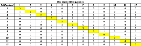
On the above crosstab, we have marked the main diagonal in yellow. For the cells on this main diagonal, the estimated LGD is the same as the observed LGD. Consequently, we can already conclude that, for discriminatory power, the more loans that are in cells on this yellow main diagonal, the better.

For this LGD crosstab, total frequency  Each cell is denoted by , so that the vector of the row totals is  and the total frequency ... The cells highlighted in yellow are those for which , also known as the main diagonal of the matrix.

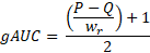
The generalized AUC can be calculated as follows:

The amounts  and  are calculated as twice the number of concordant and discordant pairs, respectively. (We will provide more details on the calculation of  and  a bit later.) The constant  is calculated as the squared number of observations minus the sum of squared row totals – so, .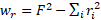

The gAUC is standardized to an outcome between 0 and 1. The closer it gets to 1, the higher the association between estimated and realized LGDs – and the better the model.

We will now proceed with our practical example.

Concordant and Discordant Pairs

The first step to calculate the gAUC is to count the number of concordant pairs and discordant pairs. The more concordant pairs, the more association there is between estimated and realized LGDs, and the higher the gAUC. So, concordant pairs have a favorable impact on the gAUC, while discordant pairs have an unfavorable impact.

Let’s start by counting the number of concordant pairs. For each cell in the matrix, we can calculate how often the estimated and realized LGDs are both higher than the estimated and realized LGDs for the loans of this cell.

When looking at the matrix of Figure 1, loans for which both estimated and realized LGDs are higher (for a specific cell) are those for which the corresponding cell  has both a higher  index and a higher  index. So, first, we need to add up all frequencies for which both indices are higher than the ones for a specific reference cell.

We then add to that the number of loans for which the estimated and realized LGDs are both lower than the estimated and realized LGDs of this given cell, as evidenced by their indices  and .

Suppose that we do this for cell (5, 5) of the matrix. To calculate the number of concordant pairs, the relevant cells to sum over are indicated below (see Figure 2) in green.

Figure 2: LGD Crosstab with Concordant and Discordant Pairs

The estimated and observed LGD pairs for which both estimated and realized LGDs are higher (or lower) than for cell (5,5) are indicated in green. Collectively, these loans are the concordant pairs for cell (5, 5).

On the other hand, the pairs highlighted in orange are the discordant pairs. As we’ve mentioned, for good discriminatory power, it is beneficial to have as many concordant pairs as possible.

The white cells are denoted as “ties.” For these ties, compared to cell (5,5), either the estimated segments are the same (i.e., both are 5) or the realized segments are the same (i.e., both are 5).

For our cell (5,5), by summing up the numbers in the green areas, we can easily verify that we have 64 (29 + 35) concordant pairs. Moreover, by summing up the numbers in the orange areas, we can see that we have 6 discordant pairs. We can also verify, from the perspective of a single loan in cell (5, 5), that we have 29 ties (see white cells).

We therefore have 99 pairwise comparisons (64 + 6 + 29) for one loan within cell (5, 5). We can repeat this procedure for all unique pairwise comparisons between the loans in all cells, and then add up all concordant, discordant and tied pairs.

For this crosstab, we arrive at the following statistics:

Figure 3: Concordance Statistics for the LGD Crosstab

As you can see above, the sum of the concordant, discordant and tied pairs is 4950. We verify this number by realizing that, for 100 loans, we can make 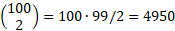 unique pairwise comparisons.

All of this data sets us up to calculate gAUC properly.

According to the ECB, and  should be calculated as twice the number of concordant and discordant pairs, respectively. Moreover, the constant  should be calculated as the squared number of observations minus the sum of squared row totals – i.e., . In our example, this is .

As a reminder, the generalized AUC is defined as:

In our example, this resolves to: .

Further Insights

We can provide further insights in the dynamics of the gAUC formula by realizing that a better (i.e., more discriminatory) LGD model will have a crosstab with higher frequencies clustered in the cells around the main diagonal (see the cells highlighted in yellow in Figure 1).

In an extreme case, for all loans, the estimated LGD segment would be equal to the realized LGD segment, and we’d have nonzero frequencies only on the main diagonal of the crosstab. In such a case, there would be no discordant pairs, and  would be zero in the gAUC formula

Moreover, would resolve to twice the number of concordant pairs. (This is a bit more difficult to see, but we will illustrate this below). Consequently, would become equal to , and the gAUC formula would resolve to:  .

Why, you might ask, would resolve to twice the number of concordant pairs? Let’s demonstrate this with the help of a smaller, [2, 2] crosstab:

For this 2-by-2 case, this crosstab would demonstrate an ideal model, in which the estimated LGD segment is always equal to the realized LGD segment – and in which there are nonzero frequencies only on the main diagonal.

Remember, now, that  is the sum of the frequencies – or, equivalently, the sum of the nonzero frequencies. So, in our (extreme) special case, would be equal to .

It then follows that . The sum of the squared row totals would be , and we'd be able to apply the formula for () to this extreme case. Moreover, since the would drop out of the equation of , we would also see that  would equal .

We have verified that, in this special case, the gAUC would be equal to 100%. Indeed, in this ideal case (which can be extended to larger crosstabs, like our initial 12-by-12 matrix), all realized LGDs would be equal to the estimated LGDs.

Parting Thoughts

The greater the correlation between estimated and realized LGDs, the better the model. Financial institutions can use gAUC – a key LGD performance metric – to help close this gap.

In this article, we have not only discussed how firms can unlock the power of gAUC but also demonstrated the importance of concordant and discordant LGD pairs. (The more concordant pairs found in a gAUC calculation, the higher the correlation between estimated and realized LGDs.) Moreover, we have shown that in an ideal LGD model, the gAUC resolves to 100% – i.e., the realized LGD segments are equal to the estimated ones.

Dr. Marco Folpmers (FRM) is a partner for Financial Risk Management at Deloitte Netherlands. The author wishes to thank Tom Greeven (M.Sc.) and Mats Mackaij (M.Sc.) for their review of a previous draft.